Kalman Filter

State Estimation

Kalman Filters (KFs) belong to a class of State Estimation algorithms. A state is a vector of variables that we care to know and that can describe the state. It means that if you know the state vector at time k and the input given to the system, you can know (using some sort knowledge of the system workings as well) the state of the system at time k+1.

We are making an important assumption here that is necessary for the KF to work: your current state only depends on the precedent. In other words, the “history” of the system state is condensed in the previous state, that is to say each state is independent from the past, given the precedent state. This is also known as Markov assumption. If this doesn’t hold, you cannot express the current state in terms of the precedent one alone.

In KFs, all the uncertainties are treated using Gaussian distributions. A Gaussian distribution is a nice way of representing something you are not really sure about. Your current belief can be represented by the mean of the distribution, while the standard deviation will say how confident you are in your belief. The uncertainty is represented as covariance matrix.

Kalman Filter Cycle

The Kalman filter represents our distributions by Gaussians and iterates on two main cycles: Prediction and Measurement update. It’s a two-step process, it first predicts information based on its current belief, then it updates its belief with new information.

Before getting into the details of the Kalman filter algorithm cycle, consider below example of estimating the car position based on the prediction result and measurement result using Kalman filter.

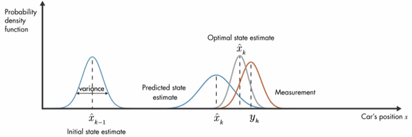
We can explain the working principles of kalman filters with the help of probability density function as shown below.

At initial time step k-1, car position can be in the mean position of gaussian distribution at xk-1 position. At the next time step K, uncertainty at xk position increases which is shown below with larger variance.

Next one is the measurement result y from the sensors and noise represented in the variance of the third Gaussian distribution as shown below.

Kalman filter says optimal way to estimate the position is combining these two results. This is done by multiplying these two probability functions together and the result will also be another Gaussian function.

Let’s get into the two cycles of Kalman filters: Prediction and Measurement update.

Implementation

Prediction Phase:

In this step the Kalman Filter predict the new values from the initial value and then predict the uncertainty/error/variance in our prediction according to the various process noise present in the system.

Our model will assume the car to move with a constant velocity due to zero acceleration but in reality it will have acceleration i.e. it speed will fluctuate from time to time. This change in acceleration of that car is the uncertainty/error/variance and we introduce it to our system using process noise.

Update Phase:

In this step we take the actual measured value from the devices of the system. In case of autonomous vehicle these devices can be radar or Lidar .We then calculate the difference between the predicted value and the measured value and then decide which value to keep i.e. predicted value or measured value by calculating the Kalman Gain. Based upon the decision made by the kalman gain we calculate the new value and new uncertainty/error/variance.

This output from the update step is again fed back to the prediction step and the process continues till the difference between the predicted value and the measured value tend to convert to zero. This calculated value will be the prediction/educated guess done by the Kalman Filter.

Kalman Gain: It determines whether our predicted or measured value is close to the actual value. It is responsible for giving the Kalman filter where to put more weight on either the predicted location or the measured location depending on the uncertainty of each value. Its value ranges from 0 to 1. If its value is near to 0 then it means predicted value is close to the actual value or if the value is near to 1 then it means final measured value is close to the actual value.

From the error perspective, if measurement error received from sensor is low, KG will be close to 1 meaning it will take larger fraction of new sensor measurement in update step; on the other hand if the error/uncertainty is more it will be close to 0 meaning it will take only a small fraction of it and incorporate in previous estimation. It is represented by the simple formula as show below.

K = Error in Prediction / (Error in Prediction + Error in Measurement)

Prediction Steps:

x′ = F.x + B.μ + ν

P′ = FPFᵀ + Q

P: Process Covariance Matrix

Models the uncertainty in the system.

F: State Transition Matrix

It is used to transform the state vector matrix from one form to another

Suppose the state of a vehicle is given by position p and velocity v and is not accelerating at time t.

X = [p, v]

After a time particular time say t+1 the new state vector X’ will be

p’ = p+v*Δt

v’=v

In matrix form this can be shown as below:

x’ = F*x

Q: Process Noise Covariance matrix

The model assumes velocity is constant between time intervals, but in reality we know that an object’s velocity can change due to acceleration. So after a time Δt, our uncertainty increases by a factor of Q which is again noise. So we add noise into noise technically.

B: Control input Matrix

Denotes the change in state of object due to internal or any external force. For example- the force of gravity or the force of friction to the object.

Why B.μ = 0?

Mostly, in the context of autonomous cars the value of control product vector is equal to zero because we cannot model the external forces acting on objects from the car.

Update Steps:

A quick recap in update step we do the following:

Step 1: Find the difference between actual measured value and predicted value

Step 2: Calculate Kalman Gain

Step 3: Based upon the result of Kalman Gain calculate new x and P.

Now we will see the mathematical implementation of these steps

Step 1:

y= z — H.x′

z: Actual measurement data

It is the actual data that is coming from the sensor.

H: State transition matrix

Sensor reading will be of form vector z = [px, py]. As stated before, we need to compare this measurement value with the value predicted in step a. But looking at both vectors (predicted state vector x and measurement vector z), we see that both are of different order. Hence to convert state matrix to same size as z, we introduce matrix “H”. Getting into matrices basics, to convert a 4 x 1 ‘x’ matrix to 2 x 1 ‘z’ matrix (while keeping top two values as it is and removing velocity variables) we use a 2 x 4 matrix H. So the equation comparing predicted value with measurement becomes y = z — Hx, which gives us the difference between both values.

Step 2:

S= HP′Hᵀ + R
K= P′HᵀS⁻¹

R: Measurement Noise

R denotes the noise in the measurement. The devices that measure the values also have some degree of inaccuracy. All devices comes with a predefined value for R parameter that is given by the manufacturer.

S: Total Error

It is the sum of the prediction error plus the measurement error.

K: Kalman Gain

Uncertainty in predicted state / (Uncertainty in predicted state + Uncertainty in measurement readings). We know uncertainty in predicted state is matrix P and that in measured value is matrix R and the total uncertainty is S. But as you can see, both of them are of different size. Hence we use H matrix to convert P matrix to correct size. Since it is matrix representation, we cannot divide so here we are taking S⁻¹.

Step 3:

x = x′ + K.y
P = (I- KH)P′

Finally we update are state vector and the covariance matrix.

Interesting points about Kalman filter

• optimal (mathematically proven… you can just believe it or understand it minimizes mean square error between estimate and real value)
• recursive (will take last set of results as input for next calculation)
• It predict the next state based on the previous state only , no need of the history of data
• light on memory (only keep data of last immediate state)
• computationally very fast making it well suitable for real time problems
• even if lots of noise/error/uncertainty occurs in the environment, Kalman filter will give a good result

Drawbacks of Kalman Filter

· A Kalman filter is only defined for linear systems.

· Kalman filters work with Gaussians or normal distribution

Summary

- Predict position and velocity with some uncertainty.
— Then measure the experimental position and velocity with some uncertainty.
— Finally, increase the certainty of our prediction by combining our prediction with the measurement information.