Particle filter

Particle filter normally carry discrete no. of particles. Each particle is a vector which contains x coordinates, y coordinates, and orientation. Particles survive based on how they are consistent with sensor measurements. The consistency is measured based on mismatch between actual measurement and predicted measurement which is called weights. Weights are the measure of how important the particles are. The larger the weight, the more important it is. The probability of survival of a particle is proportional to its weight.

Implementation

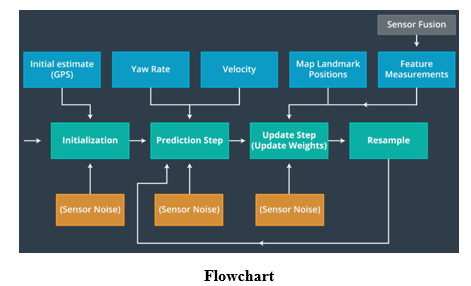
Particle filters has got four major steps:

1. Initialization step: At the initialization step we estimate our position from GPS input.
2. Prediction step: During the prediction step we add the control input (yaw rate & velocity) for all particles.
3. Update step: During the update step, we update our particle weights using map landmark positions and feature measurements.
4. Resample step: During resampling we will resample M times, drawing a particle i, proportional to its weight. Resampling wheel is used at this step.

1. Initialization step

Initialize all the particles. At this step we have to decide how many particles we want to use. It shouldn’t be too small that will prone to error or too high so that it is computationally expensive.

2. Prediction step

To predict the vehicle’s position, the below formula will be used to predict where the vehicle will be at the next time step, by updating based on velocity and yaw rate.

3. Update step

Next step is to update particle weights based on LIDAR and RADAR readings of landmarks.

Update step has got three major steps:

1. Transformation
2. Association
3. Update Weights

Transformation

The agent’s measurements need to be transformed from its local coordinate system to the map coordinate system.

Here Xm and Ym are the transformed map coordinates of the measured observations. Xp, Yp are the particles, position. Xc, Yc are the position of the observation in the agent’s local coordinate system and theta is the rotation angle through a homogenous transformation matrix.

This homogenous transformation matrix, shown below, performs rotation and translation.

Matrix multiplication results in:

Associations

Association is the problem of matching landmark measurement to object in the real world such as map landmarks. As we have multiple measurements to the landmark, we can use Nearest Neighbor technique to find the right one.

Weight Update

The ratio of the actual measurement to the predicted measurement is the called the importance weight of that particle. As the predicted measurement approaches the actual measurement, the weight gets closer to one. Thus, larger the weight, more likely the particle represents the correct vehicle position.

3. Resample step

Randomly drawing samples is not the most efficient way of resampling in terms of how many operations are involved. To make the resampling more efficient we use a technique called the resampling wheel.

Resampling is the technique used to randomly drawing new particles from old ones with replacement in proportion to their importance weights. After resampling, particles with higher weights likely to stay and all others may die out.

In order to do the resampling, Resampling Wheel technique is used.

Thus, after resampling, our particles will be much closer to the actual location of the car and will be much closer to each other hence with a reduced noise.

Particle Filter vs Kalman Filter

Particle Filters can be used in order to solve Non-Gaussian noises problems, but are generally more computationally expensive than Kalman Filters. That’s because Particle Filters uses simulation methods instead of analytical equations in order to solve estimation tasks.

The Detriment of Particle Filtering

1. When the sample size is too small, the particles may drift away and never converge in a way that the particles populate near the desired state.
2. If the sample size is too large, then the particles will collapse onto each other. It’ll look like one big point where all the particles got too attached to each other. This is cleverly called particle collapse.
3. The more complex the environment the robot faces, the more samples are needed to describe the posterior probability distribution, and the more complex the algorithm.
4. In addition, the re-sampling phase can result in loss of sample validity and diversity, leading to sample depletion.

Summary

The main aim behind particle filter is to generate a posterior probability of each particle being the actual car based on the measurement coming from the actual car and the measurement from the dummy cars (particles) and as the car continues to move, irrelevant particles will be gradually filtered out.

So in general, implementation of particle filter can be summarized in 3 steps:

1. Generating a set of particles
2. Measure the probability of each particle being the actual car(robot)
3. Resample based on the probability weight