Path Planning Algorithms
Path Planning: Finding a continuous path that connects a start configuration S and a goal configuration G, while avoiding collision with known obstacles.
Trajectory Planning: It usually refers to the problem of taking the solution from a robot path planning algorithm and determining how to move along the path. It takes into consideration the Kino-dynamic constraint to move along the specified path.
Configuration space
A configuration describes the pose of the robot relative to a fixed coordinate system, and the configuration space C is the set of all possible configurations. A pose is a vector of positions and orientations,
C-Space Construction
Increasing the size of the obstacles by blowing them up” by the robot radius and sliding the robot along the edge of the obstacle regions in all orientations. This effectively “shrinks” the robot back to a point. If the robot is a single point, configuration can be represented using two parameters (x, y).
- If the robot is a 2D shape that can translate and rotate, configuration can be represented using 3 parameters (x, y, θ).
- If the robot is a solid 3D shape that can translate and rotate, configuration requires 6 parameters: (x, y, z) for translation, and Euler angles (α, β, γ).
- If the robot is a fixed-base manipulator with N revolute joints (and no closed-loops), C is N-dimensional.
Grown Obstacle

1. Find a set of vertices that determine the grown obstacle.
2. Reflect the robot about its X and Y axes.
3. Placing this reflected object at each obstacle vertex. This constitutes a grown set of vertices.
4. Given the grown set of vertices, find its convex hull and form a grown polygonal obstacle.
Note: For a set of points {1, 2, 3….S}, the convex hull is an enclosing polygon in which every point in S is in the interior or on the boundary of the polygon. A test for convexity: Given a line segment between any pair of points inside the Convex Hull, it will never contain any points exterior to the Convex Hull.

For Concave shaped robot A, decompose into convex regions and compute the grown space of each convex region with obstacle B and union the resulting grown spaces.

Find the path after increasing the size of the obstacle.

Free space
The set of configurations that avoids collision with obstacles is called the free space Cfree. The complement of Cfree in C is called the obstacle region.
Obstacle space
Obstacle space is a space that the robot cannot move to.
Path Planning Algorithm Properties
· Completeness: An algorithm is said to be complete it finds it in finite time whether a path exists or does not exist.
· Sound: An algorithm is said to be sound if it is guaranteed to never cross an obstacle.
· Optimal: An algorithm is said to be optimal if it is guaranteed to find the shortest path (if it exists).
Active & Passive Algorithms
Active algorithms can achieve the best feasible path to the goal all by its own processing procedure. Passive algorithms only generate a set of safe paths from start to the goal but cannot find the optimal shortest path from start configuration to goal configuration.
Algorithms
The Continuous terrain needs to be discretized for path planning. There are various approaches to discretize C-spaces. Low-dimensional problems can be solved with grid-based algorithms that overlay a grid on top of configuration space, sampling-based algorithms are currently considered state-of-the-art for motion planning in high-dimensional spaces.
Interval-based algorithms
These approaches are similar to grid-based search approaches except that they generate a paving covering entirely the configuration space instead of a grid. The paving is decomposed into two subpavings X−, X+ made with boxes such that X− ⊂ Cfree ⊂ X+.
The robot is thus allowed to move freely in X−, and cannot go outside X+. To both subpavings, a neighbor graph is built and paths can be found using algorithms such as Dijkstra or A*. When a path is feasible in X−, it is also feasible in Cfree. When no path exists in X+ from one initial configuration to the goal, we have the guarantee that no feasible path exists in Cfree. As for the grid-based approach, the interval approach is inappropriate for high-dimensional problems, due to the fact that the number of boxes to be generated grows exponentially with respect to the dimension of configuration space.
Reward-based algorithms
Here outcomes (displacement) are partly random and partly under the control of the robot. The robot gets positive reward when it reaches the target and gets negative reward if it collides with an obstacle.
Sampling-based algorithms
Sampling-based algorithms abandons the concept of explicitly characterizing Cfree and Cobs and leave the algorithm in the dark when exploring Configuration space and uses collision-detection to probe and incrementally search the C-space for solution. It represents the configuration space with a roadmap of sampled configurations. A roadmap is then constructed that connects two milestones P and Q if the line segment PQ is completely in Cfree. Again, collision detection is used to test inclusion in Cfree.
These algorithms work well for high-dimensional configuration spaces, because unlike combinatorial algorithms, their running time is not (explicitly) exponentially dependent on the dimension of C. They are also (generally) substantially easier to implement. They are probabilistically complete, meaning the probability that they will produce a solution approaches 1 as more time is spent. However, they cannot determine if no solution exists. It is neither complete nor optimal.
3D Voronoi
It forms a 3D obstacle free network based on pre-known knowledge of the whole environment, which contains obstacle and free regions. It samples the space and extracts the place with the maximal clearance from all nearest obstacles. It cannot generate the shortest path at the same time. Thus it seeks help from Dijkstra’s algorithm, A*, D*. It also suffers from unnatural attraction to open space, suboptimal paths.
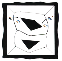
Steps to Voronoi path generation methods: (a) Sampling the environment (b) Generating a 3D Voronoi graph © Find point Qstart’ on the Voronoi graph closest to Qstart (d) Find point QGoal’ on the Voronoi graph closest to QGoal © Employing a search algorithm to find the minimal cost path globally between Qstart’ and QGoal’.
Visibility graphs
A an undirected graph G = (V, E) where the V is the set of vertices of the grown obstacles plus the start and goal points, and E is a set of edges consisting of all polygonal obstacle boundary edges, or an edge between any 2 vertices in V that lies entirely in free space.
Visibility graph constructs a path as a polygonal line connecting start configuration S and a goal configuration G through vertices of obstacles.
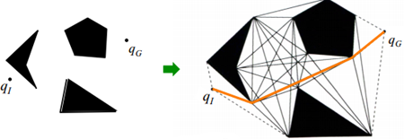
Steps to create a Visibility Graph: (a) Find nodes: Nodes are start point, goal point, vertices of obstacles (b) Connect all nodes which are “visible” — straight line un-obstructed path between any 2 nodes © check each edge to see if it intersects any of the grown obstacle edges in the graph If so, reject this edge. The remaining edges (including the grown obstacle edges) are the edges of the visibility graph (d) search for path from start to goal using search algorithm.
Advantage: Can generate optimal shortest paths (based on path length) –Disadvantage: Can cause robot to move too closely to obstacles (solution: grow obstacles even more, to give more open space between robot and obstacle)
Cell Decomposition-based algorithms
It discretize the configuration space into cells so that any path inside a cell is obstacle free. It is of two types: Exact and Approximate
Approximate Cell Decomposition
It defines a discrete grid in C-Space by marking any cell in the grid as Cobs or Cfree depending whether the cell is containing any obstacles or not. It finds path through remaining cells by using any search algorithm.
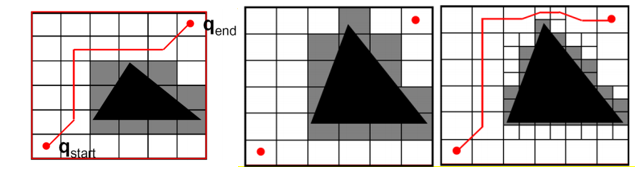
If it cannot find a safe path, it first distinguish between cells that are entirely contained in Cobs (FULL) and cells that partially intersect Cobs (MIXED), then it subdivides the MIXED cells to produce new set of free cells and again tries to find a path using the current set of free cells.
Exact Cell Decomposition
Divide the configuration space into cells. Steps to perform Exact Cell Decomposition: (a) Draw vertical lines running up and down along the vertices of the obstacles (b) Find midpoints or centroid of each segment formed due to consecutive line segments or between the line segment and the obstacle boundary © Connect all such centroids. These become the edges (d) search for path from start to goal through the edge formed using search algorithm.
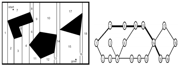
Cell Decomposition methods are inefficient for complex problems
Artificial Potential Field
Artificial Potential field methods are based on the idea of assigning a potential function (relationship between obstacle free and obstacle space) to free space and simulating the vehicle as a particle reacting to force due to the potential field. It assumes robot and obstacle to be having same polarity of electric potential whereas goal to be having opposite polarity. This implies that robot is repelled by obstacle and attracted by goal. The potential field can be represented as:
𝑈t (𝑋) =𝑈a (𝑋) + 𝑈r (𝑋), Where 𝑈t (𝑋) is the total potential at state 𝑋, 𝑈a (𝑋) is the attractive potential at state 𝑋, and 𝑈r (𝑋) denotes the repulsive potential at state 𝑋.
Robot moves in the direction of resultant of all force vectors acting on it. Robot’s velocity decreases as it moves closer to goal and it stops when distance becomes zero.
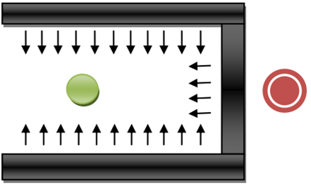
This method falls into a trap when robot reaches a point of local minima. It is a point other than destination point where resultant of all the forces is zero. This situation is depicted in the diagram where robot is shown in green color and destination point in red. It needs the whole work space sampling in formation to escape from local minima.
Potential-field algorithms are not suitable for solving real-world complex problem. Further these type of methods are incomplete because they are prone to drop into local minima area.
Summary
1. Construct configuration space (by growing obstacles to the size of the objects)
2. Select representation of configuration space either Probabilistic Road Map, Visibility Graph, Cell Decomposition or Artificial Potential Field.
3. Plan path using path planning algorithm like Dijkstra, A*, RRT, LPA*, D* or D* Lite.
Challenges in Path Planning
· High dimensionality of the configuration space.
· Continuous nature of configuration space.
· Dynamic environments (i.e. with lots of moving objects or people)
· Camera Issues : Non-smooth movements of the camera, occlusions, transparency and reflection
· Computation time, memory, sensory device and motion constraints.